Modelling Single-Vehicle Crash Occurrences on Indonesian Toll Roads

Introduction

Single-vehicle crashes, particularly run-off-road crashes, are a major cause of road fatalities worldwide (UNECE, 2021) and a major concern for highway transportation due to their potential to result in severe casualties and substantial economic losses (Xiong & Chen, 2024). In Indonesia, approximately 20 percent of road fatalities were caused by vehicle leaving the roadway and colliding with a fixed object (IIHS, 2015). Given the nature of single-vehicle crashes, road characteristics and roadside infrastructure play a significant role in enhancing road safety by preventing crashes minimising harm (Duddu et al., 2020).

Previous studies have highlighted several road and traffic characteristics that contributed to higher likelihood of single-vehicle crashes. Liu and Subramanian (2009) identified that run-off-road crashes were more likely to occur on curved than on straight road segments. Marchesini and Weijermars (2010) reported that roads with higher traffic volumes experienced more single-vehicle crashes compared to roads with lower volumes. Other factors, such as vehicle speed, were linked to an increased severity of run-off-road crashes (Dissanayake & Roy, 2014). Further, Russo and Savolainen (2018) observed that freeway median - crashes were more frequent on road segments with median concrete barriers, sharper curves, narrower medians and left shoulders, as well as higher speed limit. Several engineering measures can be used to keep vehicles on the road and prevent such crashes including improving road surface conditions, installing edge line rumble strips to alert drivers who may drift off the road, and providing clear zones and crash barriers to minimise crash severity (Dissanayake & Roy, 2014; Gong & Fan, 2017; Johnston et al., 2006). However, Wu et al. (2014) concluded that while rumble strips reduced the overall number of crashes, their effect on reducing severe crash outcomes was not statistically significant.

In Indonesia, more crashes occur on toll roads (0.76 crashes per kilometre in 2019) compared to other road types (non-toll national road: 0.58, local roads: 0.17) (GRI, 2022). When considering road tolls in total, combining urban and rural segments, most crashes involve multiple vehicles, but on rural toll roads, single-vehicle crashes are more prevalent. During 2019-2020, a total of 2,295 crashes occurred on 347-km length Cikopo to Semarang section of Trans Java rural toll road, resulting in 554 fatalities and 614 serious injuries. Over half were single-vehicle crashes (58%).

To study the relationship between crash occurrences and their influencing factors, a crash prediction model or safety performance function (SPF), can be developed. Studies have indicated that there are differences in road-related factors associated with single-vehicle crashes and multi-vehicle crashes (K. Wang et al., 2017; X. Wang & Feng, 2019) making it essential to model single-vehicle crashes and multi-vehicle crashes separately (Geedipally & Lord, 2010; X. Wang & Feng, 2019; Yu et al., 2013). While crash prediction models have been developed for Indonesian toll roads (Kusumawati & Rakhmat, 2011; Rakhmat et al., 2012), they were for total crashes and did not differentiate by crash type. Further, no crash prediction model studies have focused on single-vehicle crashes on toll roads in Indonesia. It should be noted that driving behaviour in Indonesia differs from that in high income countries, where most studies on crash prediction models have been conducted. In particular, Indonesian drivers tend to disregard posted speed limits. Kusumawati and Hajidah (2024) reported the posted speed limit on toll roads is 100 km/h, yet the 85th percentile speed can reach as high as 140 km/h. This highlights the need to develop a single-vehicle crash prediction model for Indonesian toll roads that can be used to identify the associated roadway geometric and traffic factors.

The aim of this study was to investigate the road-related factors associated with single-vehicle crashes on the toll roads with the highest number of crashes and fatality per kilometre to assist toll road operators in identifying appropriate measures to enhance road safety.

Method

To study the factors associated with single-vehicle crash occurrences on Indonesian toll roads, a safety performance function (SPF) was developed using generalised linear modelling technique. The SPF related the number of single-vehicle crashes, as the response variable, with traffic flow and various toll road geometric characteristics, as the predictor variable. Considered geometric characteristics included gradient, curve type, presence of nearby ramp, presence of median opening, type and length of roadside crash barrier, type and length of median crash barrier, presence of roadside hazard, presence of bridge pier, presence of speed reducer marking, presence of shoulder rumble strips, and pavement type.

To develop the SPF, four types of models were considered: Poisson regression model, Negative Binomial regression model, Zero-inflated Poisson (ZIP) regression model, and Zero-inflated Negative Binomial (ZINB) regression model. In developing the SPF, and the best regression model was selected among them.

Traffic crashes are rare events. The number of crashes at a specific site within a given time period is often assumed to be Poisson distributed. When modelling crash count data, a Poisson regression model is suitable when the mean and variance of the crash count data are approximately equal. However, when the data exhibit over-dispersion, the Negative Binomial (NB) regression model becomes more appropriate. In some cases, no crashes may be reported during the observation period. This can create a misleading conclusion that road segments are safe when, in fact, only some of these zero-crash sites are safe while crashes have occurred at other road segments however it was outside the observation period (Kumara & Chin, 2003; Shankar et al., 1997). The use of standard Poisson and NB regression models fail to distinguish between these two types of zero-crash observations, resulting in biased estimates. Also, an over-representation of zero-crash observations may incorrectly suggest over-dispersion, leading to the inappropriate use of an NB model. To overcome such problems, the Zero-Inflated Poisson (ZIP) or Zero-Inflated Negative Binomial (ZINB) regression models were used.

The functional form of the SPF for fitting the regression model was:

$$\mu = c \times (ADT)^{\propto} \times \exp\left( \gamma_{1}G_{1} + \gamma_{2}G_{2} + \ldots \right) \tag{1}$$

where μ is the expected crash frequency (in crashes per two-year), ADT is the average daily traffic (in vehicles per day), $G_{1}$,$G_{2}$,… are geometric factors, c is a model constant, and ∝,γ are parameters to be estimated in the model.

The SPF was developed using data from a 321-km toll road section of the Trans Java Toll Road network in Indonesia, including crash data, traffic flow data, and roadway geometric characteristics. Two years of data from 2019 and 2020 were used for crashes (fatal and injury) and traffic flow for the period were gathered from the toll road operators. Roadway geometric characteristics were extracted from Google Maps. Road segments for two directions were formed (n=642 1-km segments). A summary of descriptive statistics for the segments is presented in Table 1.

There were 23 variables used to characterise the segments for developing the SPF. The response variable was the total frequency of single-vehicle crash in two-year (NCRASH) and the other 22 variables were the candidates for explanatory variables. The exposure variable was the average of 2-year average daily traffic (LNADT) included in the model in log-normal form. The other explanatory variables were selected based on the following assumptions. Higher traffic exposure increases the likelihood of crashes. A wider median with no crash barrier may increase the likelihood of a vehicle leaving the roadway to recover and safely return to its lane, helping prevent crashes. Presence of crash barrier in wide medians may increase the possibility of single-vehicle crashes. When a crash does occur, the type of barrier plays an important role in influencing the crash severity. However, median width may have a high correlation with some type of crash barriers as narrow medians normally equipped with concrete barrier while wider medians usually have no barrier or are fitted with guardrail or cable barrier. Steeper gradients and the presence of horizontal curves may increase the likelihood of drivers losing control of their vehicles. On the other hand, ramps and median openings may reduce the risk of single-vehicle crashes but raise the chance of multi-vehicle collisions. Bridge piers and roadside hazards can make drivers feel less safe, prompting them to drive more cautiously. Traffic calming measures and speed limits encourage drivers to reduce their speed, decreasing the likelihood of losing control. Shoulder rumble strips alert drivers when they depart off their lane, helping to prevent crashes, while warning signs inform drivers of potentially hazardous road conditions. The type of pavement also affects driving behaviour, as drivers tend to reduce speed on rigid pavement compared to flexible pavement. Consequently, the likelihood of losing control is lower on rigid pavement than on flexible pavement.

The explanatory variables were then pre-selected using a correlation analysis, that is if an explanatory variable had high correlation with other explanatory variable(s) then a variable with higher correlation with the response variable is selected (Table 2). Two examples are the categorical variables developed to characterise the presence of median barrier and roadside barrier in the segments, for which TMBAR0 (Segment with no median barrier) and TRSBAR0 (Segment with no roadside barrier) were excluded. For these cases, the pre-selection process revealed that using TMBAR1, TMBAR2, and TMBAR3 were more favoured than using TMBAR0 alone as TMBAR3 has a slightly higher correlation with NCRASH rather than TMBAR0, and using TRSBAR0 was more favoured than using TRSBAR1, TRSBAR2, and TRSBAR3. Further, MEDW variable was highly correlated with TMBAR0 (r = -0.78), TMBAR1 (r = -0.72), and TMBAR3 (r = 0.83) so the MEDW variable was not used in further modelling step as the median barrier variables were more detailed and can be used as a proxy to indicate whether the median is wide or narrow.

Modelling was then carried out using NLOGIT 4.0/LIMDEP 9.0 software. Explanatory variables to be retained in the model were selected using a backward elimination procedure and the least significant variable (at 95% confidence level) was progressively eliminated one by one. This process was continued until all remaining variables were statistically significant to be retained in the model, as shown by the value of the t-statistic of the estimated parameters that should be greater than or equal to 1.96, or by P-values of the estimated coefficients that were less than or equal to 0.05. However, the intercept variable was retained in the model regardless of its significance as to remove it would create zero response when all the explanatory variables are equal to zero. Figure 1 shows the selection of the best regression model follows modelling procedure.

Figure 1.Modelling procedure

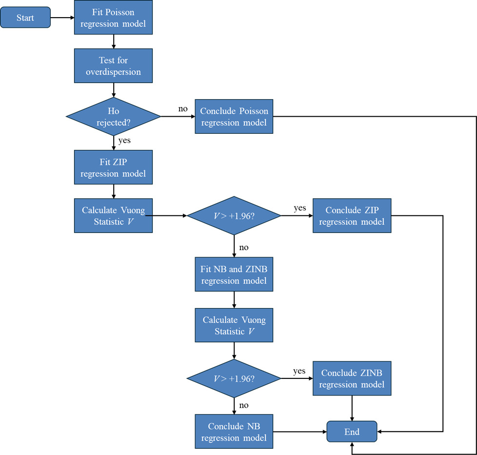
The modelling procedure started with fitting Poisson regression model. The Poisson regression model was described as follows. If $Y_{i}$ is an independent random variable that follows a Poisson distribution with expected value $\mu_{i}$, then the probability function of $Y_{i}$ is given by:

$$f(Y_{i} = y_{i}) = \frac{{\mu_{i}}^{y_{i}}\exp\left( - \mu_{i} \right)}{y_{i}!} ; i = 1, \ldots, n \tag{2}$$

where

$$E\left( Y_{i} \right) = \mu_{i} = \exp\left( {X_{i}}^{\prime}\beta \right) = \exp\left( \sum_{1}^{p}{x_{ij}\beta_{j}} \right)\tag{3}$$

and

$$Var\left( Y_{i} \right) = \mu_{i}\tag{4}$$

where $x_{ij}$ is the value of the jth covariate for observation i. In other words, $\mu\left( X_{i},\beta \right)$ denotes the function that relates the mean response $\mu_{i}$ (n x 1) to $X_{i}$ (n x p), the values of the explanatory variables for case i, and to $\beta$ (p x 1), the values of the regression coefficients.

The process continued with overdispersion test using test statistics $g\left( \mu_{i} \right) = \mu_{i}$ and $g\left( \mu_{i} \right) = \mu_{i}^{2}$. Under the null hypothesis of equidispersion, the statistics have limiting chi-squared distribution with one degree of freedom. If the null hypothesis of equidispersion is rejected, then we continued with fitting the ZIP regression model with the following form:

$$P(Y_{i} = y_{i}) = q_{i} + \left( 1 - q_{i} \right)\mspace{6mu} e^{- \lambda_{i}};\ y_i = 0 \tag{5}$$

$$P(Y_{i} = y_{i}) = \left( 1 - q_{i} \right)\frac{e^{- \lambda_{i}}{\lambda_{i}}^{y_{i}}}{y_{i}!};\ y_i = 1, \ldots, n\tag{6}$$

and

$$\log\left( \frac{q_{i}}{1 - q_{i}} \right) = \tau\sum_{1}^{p}{x_{ij}\beta_{j}}\tag{7}$$

$$\lambda_{i} = \exp\left( {X_{i}}^{\prime}\beta \right) = \exp\left( \sum_{1}^{p}{x_{ij}\beta_{j}} \right);\ i = 1, \ldots, n \tag{8}$$

where τ is a scalar parameter. The mean and variance of $Y_{i}$ were:

$$E\left( Y_{i} \right) = \mu_{i} = \left( 1 - q_{i} \right)\lambda_{i}\tag{9}$$

$$Var\left( Y_{i} \right) = \mu_{i} + \left( \frac{q_{i}}{1 - q_{i}} \right)\mu_{i}^{2} \tag{10}$$

When $q_{i} = 0$, the ZIP regression model was identical to the Poisson regression model. Also, when 0 < q_i < 1, the variance of $Y_{i}$ will exceed its mean. Thus, the ZIP regression model allows over-dispersion in the data due to excess zeros when compared to the standard Poisson regression model. When the data have excess zeros, then the ZIP regression model is preferable to NB regression model as it allows for the over-dispersion in the data due to excess zeros.

The next step was to assess the appropriateness of using the ZIP model over the Poisson model. In this case, Vuong statistic is used to assess the suitability of using the zero inflated models (ZIP or ZINB), which was computed as:

$$V = \frac{\bar{M}\sqrt{n}}{S_{M}}\tag{11}$$

where $\bar{M}$ is the mean with $M = \log\left\lbrack f_{1}(.)/f_{2}(.) \right\rbrack$, $f_{1}(.)$ being the density function to ZIP or ZINB distribution and $f_{2}(.)$ is the density function of the standard Poisson or NB distribution, $S_{M}$ and n are the standard deviation and sample size, respectively. A value of V > 1.96 (95% confidence level for the t-test) favours the ZIP or ZINB while a value of V < -1.96 favours the standard Poisson or NB distribution, and values between -1.96 and 1.96 indicate the test is indecisive (Shankar et al., 1997).

If the Vuong statistic result showed that the Poisson model is more favoured over the ZIP model, then the modelling continued with fitting the NB and ZINB models. The NB model is described as follows. If $Y_{i}$ is an independent random variable that follows a Negative Binomial distribution with expected value $\mu_{i}$, then the probability function of $Y_{i}$ is given by:

$$\scriptsize{\begin{aligned} f(Y_{i} = y_{i}) &= \frac{\Gamma\left( y_{i} + \frac{1}{\alpha} \right)}{\Gamma\left( y_{i} + 1 \right)\Gamma\left( \frac{1}{\alpha} \right)}\left( \frac{1}{1 + \alpha\mu_{i}} \right)^{\frac{1}{\alpha}}\left( \frac{\alpha\mu_{i}}{1 + \alpha\mu_{i}} \right)^{y_{i}};\\ i &= 1, \ldots, n \end{aligned}}\tag{12}$$

with $\alpha$ being the dispersion parameter, and $\alpha \geq 0$. Here,

$$E\left( Y_{i} \right) = \mu_{i} = \exp\left( {X_{i}}^{\prime}\beta \right) = \exp\left( \sum_{1}^{p}{x_{ij}\beta_{j}} \right) \tag{13}$$

and

$$Var\left( Y_{i} \right) = \mu_{i} + \alpha\mu_{i}^{2} \tag{14}$$

The ZINB regression model has the following form:

$$P(Y_{i} = y_{i}) = q_{i} + \left( 1 - q_{i} \right)\mspace{6mu}\left\lbrack \frac{1}{1 + \alpha\mu_{i}} \right\rbrack^{\frac{1}{\alpha}};\ y_i = 0 \tag{15}$$

$$\scriptsize{\begin{aligned} P\left( Y_{i} = y_{i} \right) &= \left( 1 - q_{i} \right)\left\lbrack \frac{\Gamma\left( y_{i} + \frac{1}{\alpha} \right)\left( \frac{1}{1 + \alpha\mu_{i}} \right)^{\frac{1}{\alpha}}\left( \frac{\alpha\mu_{i}}{1 + \alpha\mu_{i}} \right)^{y_{i}}}{\Gamma\left( \frac{1}{\alpha} \right)y_{i}!} \right\rbrack;\\ y_i &= 1, ..., n \end{aligned}}\tag{16}$$

with $\alpha$ being the dispersion parameter, and

$$\log\left( \frac{q_{i}}{1 - q_{i}} \right) = \tau\sum_{1}^{p}{x_{ij}\beta_{j}} \tag{17}$$

where τ is a scalar parameter.

The mean and variance of $Y_{i}$ were:

$$E\left( Y_{i} \right) = \mu_{i} = \left( 1 - q_{i} \right)\lambda_{i}\tag{18}$$

$$Var\left( Y_{i} \right) = \mu_{i} + \left( \frac{q_{i} + \alpha}{1 - q_{i}} \right)\mu_{i}^{2}\tag{19}$$

where

$$\begin{aligned} \lambda_{i} &= \exp\left( {X_{i}}^{\prime}\beta \right) = \exp\left( \sum_{1}^{p}{x_{ij}\beta_{j}} \right);\\ i &= 1, \ldots, n \end{aligned}\tag{20}$$

Finally, the appropriateness of ZINB over NB model were assessed using Vuong Statistic again. If the Vuong Statistic showed that the ZINB model was more favoured than the NB model, then it was concluded that the ZINB model was the best regression model to be used for the model. Otherwise, the NB model was selected.

Results

Table 3 shows the result of fitting Poisson regression model. Of the included variables, only LNADT, RAMP, TMBAR3, TRSBAR0, BRDG, and PVMT were significant (95% CI), as indicated by the t-statistic of all the parameters. The process continued with testing whether there is overdispersion in the data using test statistics $g\left( \mu_{i} \right) = \mu_{i}$ and $g\left( \mu_{i} \right) = \mu_{i}^{2}$. The calculation shows that $g\left( \mu_{i} \right) = \mu_{i} = 5.12$ and $g\left( \mu_{i} \right) = \mu_{i}^{2} = 5.14$. Since the critical value from the chi-squared table for one degree of freedom is 3.84, the null hypothesis of equidispersion was rejected.

The modelling continued with fitting ZIP regression model and test whether the ZIP model was more favoured than the Poisson model using Vuong statistic. The resulting ZIP model is presented in Table 4.

The Vuong statistic for testing the ZIP versus the Poisson model was calculated to be 1.82. A value of Vuong Statistic > + 1.96 favours the ZIP model over the Poisson model, while a value of Vuong Statistic < - 1.96 rejects the ZIP model. Therefore, the ZIP model is not favoured over the standard Poisson model. The modelling continued with fitting the NB model and the result is presented in Table 5.

The modelling with NB regression shows that the dispersion parameter Alpha ($\alpha$) was significantly different from zero. After the ZINB regression model was fitted into the data, and the modelling result is presented in Table 6. It turns out that the Tau ($\tau$) parameter is not significantly different from zero, and the Vuong statistic is -1.07. Therefore, the NB model is more favoured than the ZINB model.

Before concluding with the NB model, the goodness-of-fit of the NB model was compared with the standard Poisson model, as presented in Table 7.

The likelihood ratio statistic (chi-squared) for the NB model is then calculated from the likelihood function of the NB model and Poisson model, resulting the value of 113.36, which is far larger than the critical chi-squared with one degree of freedom (3.84), which means the null hypothesis is rejected. Moreover, the AIC and BIC for the NB model are smaller than that for Poisson model. Therefore, we conclude that the NB regression model is the best fit in describing the relationship between single-vehicle crashes and traffic flow and various geometric characteristics of toll roads.

Thus, the resulting SPF for single-vehicle crashes on toll roads are:

$$\scriptsize{\begin{aligned} N_{SVCR} &= 0.817 \times {ADT}^{0.276}\\ & \quad \times e^{(0.585TMBAR3 + 0.426TRSBAR0 - 0.231RAMP - 0.335BRDG - 0.345PVMT)} \end{aligned}}\tag{21}$$

where:

$N_{SVCR}$ = expected single-vehicle (fatal and injury) crashes in 2-year

$ADT$ = average daily traffic (average value in 2-year)

$TMBAR3$ = categorical variable for presence of concrete median barrier (1 = with concrete barrier present, 0 = no concrete barrier)

$TRSBAR0$ = categorical variable for no roadside barrier (1= no roadside barrier, 0 = with roadside barrier)

$RAMP$ = categorical variable for presence of ramp (1 = ramp available, 0 = no ramp available)

$BRDG$ = categorical variable for presence of bridge pier (1 = bridge pier available, 0 = no bridge pier available)

$PVMT$ = categorical variable for type of pavement surface (1 = concrete, 0 = asphalt)

The resulting SPF was validated using 2021-2023 crash data for a 115-km segment of the same toll roads used for developing the SPF, which forms as many as 230 1-km segments (accounting for two directions). Predicted single-vehicle (fatal and injury) crashes over a 2-year period were calculated for these segments and compared with the actual 2021-2023 single-vehicle (fatal and injury) crash data, which were proportionally adjusted to represent a 2-year period. The validation employed sum of squared errors (SSE) and root mean square error (RMSE) metrics. The results showed that the SSE was 416.882, and the RMSE was 3.285. The results showed that the SSE was 416.882 and the RMSE was 3.285. These values were lower than those from the initial dataset (2019–2020 crash data) used to develop the model, which had an SSE of 448.731 and an RMSE of 3.806. Therefore, it is concluded that the developed SPF model demonstrates sufficient predictive capability.

Discussion

Factors associated with single- vehicle (fatal and injury) crashes

The model identified various factors linked to single-vehicle (fatal and injury) crashes on toll roads, including average daily traffic, the presence of roadside barriers (specifically concrete barriers), presence of nearby ramp, bridge piers, and type of pavement surface.

Higher frequency of single-vehicle crashes was associated with higher average daily traffic (ADT), presence of concrete barrier, and the absence of roadside crash barriers while lower frequency of single-vehicle crashes was associated with the presence of a nearby ramp, bridge piers, and segment with rigid pavement. Factors not significantly associated with single-vehicle crashes included gradient, curve, roadside hazard, traffic calming, shoulder rumble strips, speed limit sign, and warning signs.

Average Daily Traffic (ADT)

The foremost factor affecting the frequency of single-vehicle crashes in this study was ADT, demonstrating a positive association with the frequency of single-vehicle crashes. This finding contrasts with previous studies that reported single-vehicle crashes are more likely to occur under low traffic volumes (Armstrong et al., 2008; Candappa et al., 2013). However, an increase in traffic volume generally leads to more crashes overall (Cadar et al., 2017; Chen et al., 2014), although the relationship with single-vehicle crashes remains mixed. This inconsistency may be attributed to differences in study areas, levels of data aggregation, crash types, or methodologies (Hesjevoll & Elvik, 2016). Heye (2020) also observed that the relationship between traffic volume and crash frequency tends to be stronger at higher volumes, but this effect may weaken for fatal and single-vehicle crashes. While higher traffic volumes often reduce travel speeds, the toll roads examined in this study operated well below capacity, meaning increased traffic did not significantly lower speeds. This may explain why, in this model, the higher ADT is associated with higher single- vehicle crash frequency. Previous research has shown that single-vehicle crashes often occur at low traffic volumes, with monotony and boredom being common contributing factors (Armstrong et al., 2008; Candappa et al., 2013).

The presence of barriers

Positive associations with single- vehicle crash frequency were identified with the presence of a median concrete barrier and the absence of a roadside barrier. These segments are typically situated in the central sections of the Trans Java toll road where drivers may experience increased drowsiness, thereby increasing the probability of running off-road. Further, as no clear zone was provided along the roadside, segments without a roadside crash barrier are associated with an increased number of fatal and injury single-vehicle crashes.

Median barriers can prevent out-of-control vehicles from crossing into opposing lanes and colliding with oncoming traffic. While the presence of a median barrier cannot eliminate crashes entirely, it can significantly reduce crash severity and reduce fatalities and injuries. Several studies have also reported that the frequency of median-related crashes tends to increase after the installation of median barriers, however, these crashes are generally less severe (Donnell & Mason, 2006; Hunter et al., 2001; Miaou et al., 2005; Tarko et al., 2008). In this study, concrete median barriers were associated with a higher frequency of single-vehicle fatal and injury crashes. This finding aligns with prior research that concrete median barriers have the highest probability of causing fatal or injury outcomes on impact compared to other types of barriers (Kusumawati & Freddy, 2021; Russo & Savolainen, 2018). Further research is needed to determine if this also applies to non-injury crashes as property-damage-only crashes were not included in this study.

Related to the presence of barriers with crash rates and outcomes, the offset between travel lane and the median barrier, or shoulder width could have affected to the crash rates and outcomes. Chimba et al. (2014) reported that increasing the offset between the travel lane and the median barrier reduced the likelihood of median barrier crashes. A wider offset allows drivers who lose control of their vehicle more space and time to recover, reducing the chance of collision with the barrier. Additionally, a wider offset lowers the risk of secondary crashes involving other vehicles. In some cases, a wider shoulder may imply a wider barrier offset. However, Labi et al. (2017) noted that lanes and shoulders that are too wide may negatively affect safety by giving drivers a false sense of safety, potentially encouraging reckless behaviour. Similarly, Gårder (2006) identified that wider shoulders were associated with a higher crash occurrences and proportion of severe crashes. In contrast, El-Assaly and Hempsey (2012) reported no significant relationship between lane and shoulder widths and safety on two-lane paved highways, noting that their findings may not be generalisable due to regional differences in road and driver characteristics. In this study, shoulder width was excluded from the analysis due to a lack of variability in the data, as it was consistently 1.5 metres. Given Indonesia’s distinct driving behaviours (Thibenda et al., 2022) and the inconsistent findings in previous research, the effect of shoulder width on crash rates or severity in Indonesia remains unclear.

It should be noted that the barrier itself may pose a hazard to road users so careful consideration is needed before installation. A barrier should only be installed if a collision with the hazard would likely result in more severe consequences than a collision with the barrier. According to Zou and Tarko (2016), drivers who lose control of their vehicle are less likely to cross an unprotected median (i.e., one without barriers) if the median is wide, typically between 15 and 24 metres, compared to narrower medians of 9 to 15 metres. If the median is wider than the required clear zone for the operating speed and traffic volume, it may be safer and more practical to leave it unprotected. However, the risk of median cross-over cannot be eliminated, therefore providing a barrier on this wider median, such as a cable-barrier, may increase safety. Additionally in locations where cost is a factor, compared to providing a wide median, installing a barrier may be a more cost-effective safety solution.

The presence of ramp and bridge pier

In this study, the presence of a nearby ramp and unprotected bridge piers were associated with a lower frequency of single-vehicle crashes. This is likely due to reduced vehicle speeds as drivers perceive these areas as potentially hazardous. Although the presence of nearby ramps on the segments typically introduces conflicting movements between freeway traffic and vehicles entering or exiting, conditions that generally increase the likelihood of multi-vehicle crashes, this pattern was not observed on the studied toll roads. Data collected within a 500-metre range before and after the start of entry and exit ramps show that the number of multi-vehicle crashes was not significantly higher than that of single-vehicle crashes. This finding contrasts with previous research that has shown that the presence of ramps or being within a ramp influence area can result in up to a four-fold increase in crash frequency (Laflamme et al., 2022). Another study reported that ramps and their merging areas pose a high risk of crashes and conflicts due to frequent lane-changing, complex geometric designs, and variability in driver behaviour (J. Zhu & Tasic, 2021).

However, the relationship between unprotected bridge piers and crash occurrences has received limited attention in the literature. Most studies on bridge pier safety have focused primarily on the severity of crashes involving piers rather than their frequency. McDonald (2009) reported that unprotected piers are associated with significantly higher crash severity, with over 26 percent of such crashes resulting in incapacitating or fatal injuries compared to 8.5 percent when piers are protected. Similarly, Truong (2022) found that bridge-related crashes account for less than 1 percent of total crashes in Victoria and New South Wales, Australia; however, their fatality rate tends to be higher than that of non-bridge-related crashes.

Type of pavement surface/skid resistance

Pavement surface quality, particularly roughness and skid resistance, has been shown to significantly influence crash risk. Pavement friction plays an important role in highway safety as higher friction levels are generally associated with lower crash frequencies, while increased roughness correlates with higher crash rates (Cafiso et al., 2021; Chan et al., 2010; Mkwata & Chong, 2022) while improved skid resistance tends to reduce crash risk. Earlier research noted that increased roughness may reduce the risk of single-vehicle crashes, possibly due to changes in driver behaviour (Buddhavarapu et al., 2013; Karan et al., 1976). Similarly, Mayora and Piña (2009) observed that higher skid resistance lowers crash risk in both wet and dry conditions. As inadequate friction increases the likelihood of skidding or hydroplaning, especially in wet conditions, lengthening stopping distances and reducing vehicle control (Zhao et al., 2022).

In terms of pavement type, concrete pavements generally offer better skid resistance but tend to have higher roughness than asphalt pavements and asphalt pavement is considered to be safer than concrete pavement (He et al., 2024). Increased roughness can lead to reduced ride comfort, which may prompt drivers to reduce speed and exercise greater caution, potentially lowering crash risk. Better skid resistance improves tire, pavement friction, thereby further reducing the likelihood of crashes (X. Zhu et al., 2020). In contrast, asphalt pavements typically have lower roughness, which may encourage higher vehicle speeds. When combined with lower skid resistance, this can increase the risk of drivers losing control, making asphalt surfaces potentially more hazardous than concrete in certain conditions.

Study strengths and limitations

Through the SPF model, this study analysed 22 factors associated with single-vehicle crashes on toll road in Indonesia. By identifying the factors associated with single-vehicle crashes, the findings provide clarity for governments and stakeholders to identify the most effective countermeasure in high-risk segments to reduce crash risk and improve road safety outcomes.

While the SPF model is valuable for examining factors associated with single-vehicle occurrences, there are inherent limitations. First, the model is not causative. Explanatory variables should not be considered as direct causes of single-vehicle crashes rather, they represent factors associated with such crashes. Second, certain variables were omitted from the model due to minimal or no variations, this limited the scope of factors considered, including shoulder width. Third, the model’s reliance on 1-km segments may mean the effect of isolated hazardous features was submerged or lost.

The model was fitted using data from 2019-2020, and validation was conducted using data from 2021-2023. It is important to note that the years 2020 and 2021 were affected by the COVID-19 pandemic, during which full or partial lockdowns significantly reduced average traffic volumes. However, for the toll roads examined in this study, despite the decrease in traffic, the frequency of crashes increased relative to the traffic volume during the pandemic. As a result, the crash rate during the COVID period was higher compared to the normal (pre-pandemic) period. Since the model was fitted using data that partially overlapped with the pandemic period, the 2021 data, which was also affected by the pandemic, was included in the validation phase, along with the 2022 and 2023 data. This approach was taken to account for the year-to-year variability inherent in crash data and to support a more comprehensive validation. However, as more post-pandemic data become available, the model may need to be revalidated and recalibrated to eliminate the influence of the COVID-19 period and ensure its continued reliability.

Conclusions

This study identified several factors associated with fatal and injury single-vehicle crash occurrences on toll roads. Higher average daily traffic, segments with median concrete barrier and segments without roadside crash barrier are associated with a higher frequency of single-vehicle crashes. Conversely, the presence of a nearby ramp, bridge piers, and segments with rigid pavement are associated with a lower frequency of single-vehicle crashes.

Higher average daily traffic means higher exposure to crashes, thereby increasing the number of single-vehicle crashes, particularly on undersaturated road. While median barriers help prevent vehicles from crossing into oncoming lanes, they do not stop drivers of out-of-control vehicles from crashing. However, median barriers can substantially reduce crash severity and lower the number of fatalities and serious injuries. Segments lacking roadside crash barriers are linked to a higher fatal and injury single-vehicle crashes due to the absence of a clear recovery zone along the roadside.

The presence of a nearby ramp and unprotected bridge piers were associated with fewer single-vehicle crashes, likely due to reduced vehicle speeds as drivers perceive these areas as potentially hazardous. Although the presence of nearby ramps on the segments typically introduces conflicting movements between freeway traffic and vehicles entering or exiting conditions that generally increase the likelihood of multi-vehicle crashes, this pattern was not observed on the studied toll roads.

Concrete pavements generally offer better skid resistance but tend to have higher roughness than asphalt pavements. Increased roughness can lead to reduced ride comfort, which may prompt drivers to reduce speed and exercise greater caution, potentially lowering crash risk. Better skid resistance improves tyre, pavement friction and potentially further reducing the likelihood of crashes. In contrast, asphalt pavements typically have lower roughness, which may encourage higher vehicle speeds. When combined with lower skid resistance, this can increase the risk of drivers losing control, making asphalt pavement potentially more hazardous than concrete in certain conditions.

It is important to note that this study provides interesting insights related to the factors associated with single-vehicle crashes on high-speed roads. The findings may assist road operators in identifying high-risk segments for single-vehicle crashes, enabling them to take appropriate measures to reduce the risk and enhance road safety. Authorities may consider wider medians instead of narrow medians with concrete barriers. However, while wider medians can improve safety, the risk of median crossovers cannot be eliminated and installing a barrier (e.g., cable barrier) within the wider median may further enhance safety. Although constructing wide medians often involves significant investment costs, making the installation of a safety barrier a potentially more cost-effective alternative. Furthermore, installing crash barriers along the roadside is recommended to reduce the occurrence of fatal and injury-related single-vehicle crashes.

Acknowledgements

The authors would like to thank P2MI ITB for providing research grant. Portions of this research were previously presented in the form of a conference paper at the Australasian Road Safety Conference (ARSC) 2023. I would like to thank the organisers and participants for their valuable feedback during the event.

AI tools

ChatGPT 4.0 was used to improve English expression and clarity.

Author contributions

Aine Kusumawati: conceptualisation, supervision, methodology development, data analysis, result interpretation, writing, review and editing paper. Kardina N.S. Ayuningtyas: writing, literature review, review and editing paper. Istyana Hadiyanti: data preparation, model development. All authors have read and agreed to the published version of the manuscript.

Funding

The research received funding from P2MI research, Institut Teknologi Bandung.

Data availability statement

Crash data is available, on request, from the Trans Java Toll Road operators. Road geometrics/characteristics were extracted from google maps.

Conflicts of interest

The authors declare that there are no conflicts of interest.

Australasian Road Safety Conference 2023

Portions of this paper were first submitted in an Extended Abstract to the Australasian Road Safety Conference 2023 (ARSC2023) held in Cairns, Queensland, Australia from 19 to 21 September. The anonymised peer-review process recommended that Extended Abstract be accepted as an Oral Presentation and the Extended Abstract was published in the ARSC2023 Proceedings. This paper extends the Extended Abstract and was underwent further peer-review by two independent subject matter experts. This paper includes content already published in the ARSC2023 Proceedings and is reproduced here with permission.